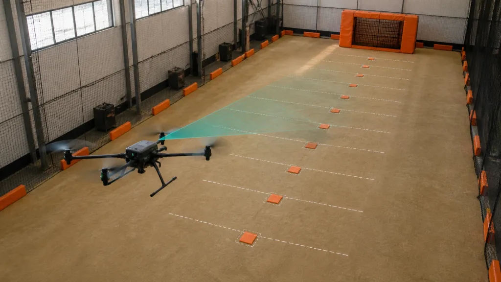
Quick answer: Drone obstacle avoidance distance is not the sensor’s maximum range. A practical minimum detection distance is the sum of distance traveled during measured sensing/control delay, braking distance at the verified deceleration, required final separation, and an uncertainty margin. Calculate it for the worst approved speed and condition, then prove it with logged tests and a safe target.
A practical drone obstacle avoidance distance model
For a straight approach with approximately constant deceleration, begin with:
D_required = v × t_pipeline + v² / (2a_verified) + D_separation + D_uncertainty
Here v is the maximum approved closing speed, t_pipeline is the measured worst-case delay from scene exposure to effective vehicle response, a_verified is conservative achieved deceleration in that condition, D_separation is the distance the aircraft must retain after stopping, and D_uncertainty covers defined measurement, control, target, and test uncertainties. This is a planning model, not a guarantee. Curved paths, acceleration limits, jerk limits, wind, attitude change, lateral motion, and estimator behavior may require a dynamic model or simulation.
PX4’s current Collision Prevention documentation explicitly accounts for controller acceleration/jerk behavior and a configurable delay. That reinforces the central point: the stop envelope belongs to the aircraft-control system, not to the range sensor alone.
Measure the inputs instead of guessing them
| Input | How to obtain it | Conservative treatment |
|---|---|---|
| Closing speed v | Synchronized vehicle-state log at approach | Use the highest approved relative speed, including relevant wind/target motion |
| Pipeline delay | Timestamp exposure/output, host receipt, obstacle update, command, and response | Use a high percentile or defined worst observed value plus justified allowance |
| Verified deceleration | Repeated restrained stops with the production control tune and payload | Use the weakest accepted result in the applicable condition |
| Final separation | Operational safety requirement and target/aircraft geometry | Include propeller radius and position uncertainty where relevant |
| Uncertainty margin | Sensor scatter/dropouts, clock error, estimator/control variation, target effects | Itemize; do not hide all unknowns in one arbitrary number |
Pipeline delay is longer than one frame interval. It can include exposure/aggregation, output scheduling, transport buffering, parsing, coordinate transform, temporal filtering, obstacle-map update, controller cycle, actuator response, and vehicle dynamics. Measure those landmarks in one synchronized log. The LiDAR data-contract guide explains the timestamp and invalid-data fields needed for that trace.
Define closing speed in the obstacle frame. A drone flying at 2 m/s toward a vehicle moving toward it at 1 m/s has a 3 m/s closing rate before avoidance. For a stationary indoor target, vehicle ground speed may be a sufficient input; for moving objects or wind-sensitive cases, document the chosen frame and assumptions.
Two worked calculations
Example A: restrained indoor approach
Assume—not measure—a 2.0 m/s approach, 0.25 s worst-case pipeline delay, 1.5 m/s² verified deceleration, 0.50 m final separation, and 0.20 m uncertainty allowance. Delay travel is 0.50 m. Idealized braking distance is 2²/(2×1.5) = 1.33 m. The planning requirement is therefore 0.50 + 1.33 + 0.50 + 0.20 = 2.53 m.
The numbers illustrate the method only. Replace every value with results from the actual vehicle, payload, controller tune, target matrix, and operating condition.
Example B: faster approach
At an assumed 4.0 m/s, 0.30 s delay, 2.0 m/s² deceleration, 0.70 m separation, and 0.30 m uncertainty, delay travel is 1.20 m and idealized braking distance is 4.00 m. Required distance becomes 6.20 m. Doubling speed did much more than double the braking term because it grows with speed squared.
If the sensor outputs at 10 fps, the aircraft moves 0.20 m per nominal frame at 2 m/s and 0.40 m per frame at 4 m/s—before other delays. This is why update rate, latency, and speed must be evaluated together.
Compare the requirement with usable sensor range
“Usable” means the project’s pass criteria are met for the target, angle, illumination, motion, mounting, and data path. It may be shorter than a published maximum. The usable range must begin before D_required and remain valid through the handoff to braking; the minimum range and close-zone behavior also need evaluation.
The Featured MRP-LD1 compact dToF module lists separate 0.5–25 m indoor and 0.2–8 m outdoor ranges. Do not substitute the indoor value into an outdoor calculation or treat the outdoor endpoint as a guaranteed detection distance for every target. Use the product values to define the outer test bounds, then establish an operational range for each critical condition.
| Verified product field | MRP-LD1 published value | Integration meaning |
|---|---|---|
| Ranging principle | SPAD direct time of flight (dToF) | Produces depth measurements; avoidance decisions remain in the host stack |
| Emitter | 940 nm VCSEL | Include target and sunlight tests at the actual mounting geometry |
| Depth output | 40 × 30 at 10 fps | Treat it as a depth grid, not as a single guaranteed stop signal |
| Field of view | 60° horizontal × 45° vertical | Map the mounted FoV into vehicle sectors and document uncovered directions |
| Published range | Indoor 0.5–25 m; outdoor 0.2–8 m | Keep indoor and outdoor envelopes separate; qualify usable range by target and light |
| Ambient-light resistance | 80 klux | A specification to test under a defined matrix, not permission to skip bright-scene validation |
| Interfaces | UART, UVC, UDP | Select a transport that the host can timestamp, parse, health-check, and replay |
| Power and mass | 5 V, 1.2 W, 8 g | Budget regulator, cable, mount, compute, and protection in addition to the module |
| Software support | Windows, ARM, Linux, Android | Confirm the required SDK build and data path on the target computer |
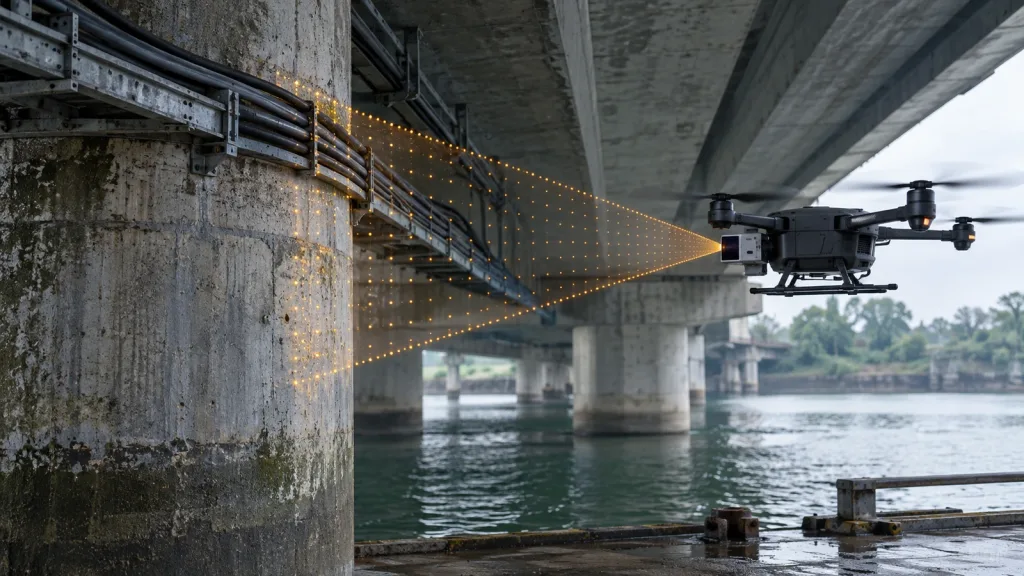
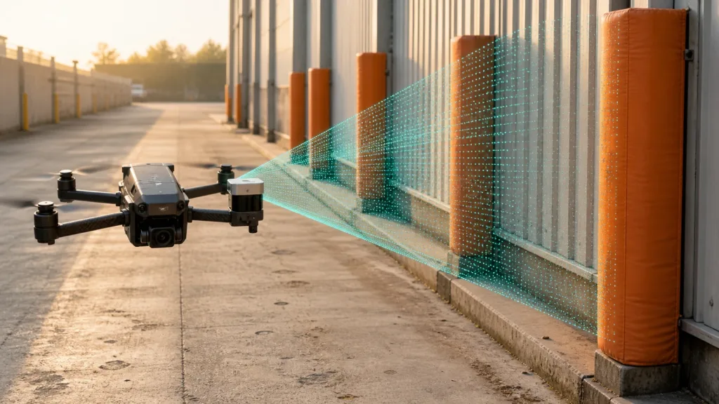
A 40 × 30 frame gives spatial samples across the FoV. Your host must decide how pixels become obstacle sectors, which invalid/low-confidence patterns block motion, and how long a sector remains fresh. The official MAVLink OBSTACLE_DISTANCE definition documents angular bins, minimum/maximum distance, increment, offset, and frame fields; preserve unknown values rather than silently converting them to clear space.
A staged brake-margin acceptance test
- Freeze the model: version the equation, inputs, allowed modes, target set, and pass thresholds.
- Calibrate the lane: measure target position, lane distances, clocks, and vehicle reference point.
- Bench the data chain: replay raw frames and verify timestamps, units, orientation, invalid values, and obstacle bins.
- Measure latency: use synchronized evidence from sensor observation to physical deceleration.
- Measure deceleration: repeat with production mass, battery state, controller tune, and relevant airflow.
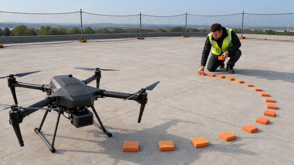
- Start below envelope: use a tether/net and soft target at low speed and generous distance.
- Expand one variable: increase speed, reduce starting distance, vary target, or change light—never all simultaneously.
- Confirm final separation: evaluate worst accepted run, not only the average.
Log raw sensor output, host timestamps, selected obstacle distance, invalid counts, vehicle pose/velocity, commanded acceleration/velocity, actuator state if available, and final separation. Video is useful for review but should not be the only evidence. For a broader sequence, see the dToF obstacle-avoidance evaluation workflow.
Test faults, sector edges, and motion the simple formula misses
Run stale timestamps, dropped packets, frozen distances, all-invalid frames, sensor reboot, host overload, controller mode change, and loss of one sector. Cross a target at the edge of the FoV and approach while yawing or pitching. A forward sensor may point downward during braking and reduce look-ahead exactly when margin is needed. The site’s forward sensing coverage guide covers that geometry.
ArduPilot’s Simple Object Avoidance documentation is also a reminder to verify the behavior of the actual flight mode and proximity configuration. The same distance stream can produce different outcomes depending on the stack, mode, parameters, and pilot command.
Common distance mistakes
- Using maximum range as stop distance: establish usable range by condition.
- Counting only braking distance: add end-to-end delay travel, final separation, and uncertainty.
- Using nominal deceleration: measure the production aircraft and choose a conservative value.
- Using average latency: tail latency and stale frames can control the safety case.
- Ignoring minimum range: prove behavior through the near zone and after the first detection.
- Testing one wall: include small, dark, angled, partial, and sector-edge targets.
- Changing many variables at once: staged expansion makes failures diagnosable.